| Visions of Chaos 3D Strange Attractor Tutorial |
|---|
|
Strange Attractors are plots of simple formulas. They are created by repeating (or iterating) a formula over and over again and using the results at each iteration to plot a point. The result of each iteration is fed back into the equation. After millions of points have been plotted fractal structures appear. The repeated points fall within a basin of attraction (they are attracted to the points that make up these shapes) rather than truly being random points over the image. If you were to plot the results of these repeated calculations as a series of numbers they would appear almost random, but once visualised as a 3D plot to the screen, you can see the complexity these very simple equations can produce. For the more mathematically inclined there is more detail here. |
| Getting Started |
|---|
 Tip: The simplest way to get started with the 3D Strange Attractors is to select an Attractor Type and then click the Search button. The Search button repeatedly tries random parameters until a set of parameters is found that will create an attractor shape. The search algorithm is based on calculating the Lyapunov exponent for the attractors. Tip: The simplest way to get started with the 3D Strange Attractors is to select an Attractor Type and then click the Search button. The Search button repeatedly tries random parameters until a set of parameters is found that will create an attractor shape. The search algorithm is based on calculating the Lyapunov exponent for the attractors.The actual paramters for the attractor equations are hidden from you, but seeing as there are up to 104 parameters for some of these attractors I purposely hide all these values to make it simpler to use. When you start the 3D Attractors mode in Visions Of Chaos the Attractors dialog has an Attractor Type dropdown at the top of the dialog. The following sections detail the formula types available. The a3da[0], a3da[1], etc are the parameter values that create the unique attractor shapes. |
| Quadratic |
|---|
|
The algorithm used to calculate the new x, y and z points is xnew=a3da[0] + a3da[1] * x + a3da[2] * y + a3da[3] * z + a3da[4] * x * x + a3da[5] * x * y + a3da[6] * x * z + a3da[7] * y * y + a3da[8] * y * z + a3da[9] * z * z ynew=a3da[10] + a3da[11] * x + a3da[12] * y + a3da[13] * z + a3da[14] * x * x + a3da[15] * x * y + a3da[16] * x * z + a3da[17] * y * y + a3da[18] * y * z + a3da[19] * z * z znew=a3da[20] + a3da[21] * x + a3da[22] * y + a3da[23] * z + a3da[24] * x * x + a3da[25] * x * y + a3da[26] * x * z + a3da[27] * y * y + a3da[28] * y * z + a3da[29] * z * z Here are some sample images created using this attractor type 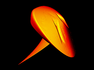 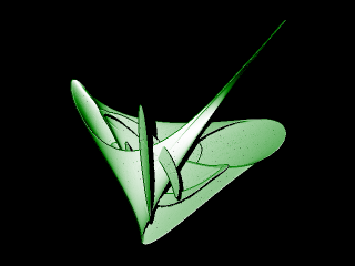 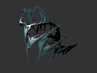 |
| Cubic |
|---|
|
The algorithm used to calculate the new x, y and z points is xnew= a3da[0] + a3da[1] * x + a3da[2] * y + a3da[3] * z + a3da[4] * x * x + a3da[5] * x * y + a3da[6] * x * z + a3da[7] * y * y + a3da[8] * y * z + a3da[9] * z * z + a3da[10] * x * x * x + a3da[11] * x * x * y + a3da[12] * x * x * z + a3da[13] * x * y * y + a3da[14] * x * y * z + a3da[15] * x * z * z + a3da[16] * y * y * y + a3da[17] * y * y * z + a3da[18] * y * z * z + a3da[19] * z * z * z ynew= a3da[20] + a3da[21] * x + a3da[22] * y + a3da[23] * z + a3da[24] * x * x + a3da[25] * x * y + a3da[26] * x * z + a3da[27] * y * y + a3da[28] * y * z + a3da[29] * z * z + a3da[30] * x * x * x + a3da[31] * x * x * y + a3da[32] * x * x * z + a3da[33] * x * y * y + a3da[34] * x * y * z + a3da[35] * x * z * z + a3da[36] * y * y * y + a3da[37] * y * y * z + a3da[38] * y * z * z + a3da[39] * z * z * z znew= a3da[40] + a3da[41] * x + a3da[42] * y + a3da[43] * z + a3da[44] * x * x + a3da[45] * x * y + a3da[46] * x * z + a3da[47] * y * y + a3da[48] * y * z + a3da[49] * z * z + a3da[50] * x * x * x + a3da[51] * x * x * y + a3da[52] * x * x * z + a3da[53] * x * y * y + a3da[54] * x * y * z + a3da[55] * x * z * z + a3da[56] * y * y * y + a3da[57] * y * y * z + a3da[58] * y * z * z + a3da[59] * z * z * z Here are some sample images created using this attractor type 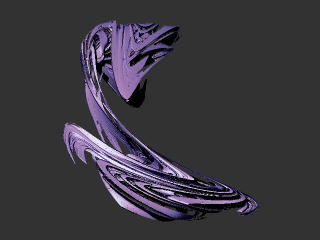 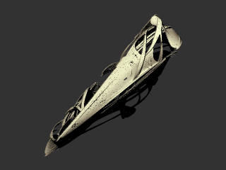 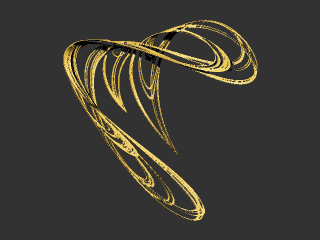 |
| Quartic |
|---|
|
The algorithm used to calculate the new x, y and z points is xy=x*y xz=x*z yz=y*z x2=x*x y2=y*y z2=z*z x2y=x2*y x2z=x2*z y2x=y2*x y2z=y2*z z2x=z2*x z2y=z2*y x3=x*x2 y3=y*y2 z3=z*z2 xyz=x*y*z x3y=x3*y x3z=x3*z y3x=y3*x y3z=y3*z z3x=z3*x z3y=z3*y x2y2=x2*y2 x2z2=x2*z2 y2z2=y2*z2 z2xy=x*y*z2 y2xz=x*z*y2 x2yz=y*z*x2 x4=x3*x y4=y3*y z4=z3*z xnew= a3da[0] + a3da[1]*x + a3da[2]*y + a3da[3]*z + a3da[4]*x2 + a3da[5]*xy + a3da[6]*xz + a3da[7]*y2 + a3da[8]*yz + a3da[9]*z2 + a3da[10]*x3 + a3da[11]*x2y + a3da[12]*x2z + a3da[13]*y2x + a3da[14]*xyz + a3da[15]*z2x + a3da[16]*y3 + a3da[17]*y2z + a3da[18]*z2y + a3da[19]*z3 + a3da[20]*x4 + a3da[21]*y4 + a3da[22]*z4 + a3da[23]*x3y + a3da[24]*x3z + a3da[25]*y3x + a3da[26]*y3z + a3da[27]*z3x + a3da[28]*z3y + a3da[29]*x2y2 + a3da[30]*y2z2 + a3da[31]*x2z2 + a3da[32]*x2yz + a3da[33]*y2xz + a3da[34]*z2xy ynew= a3da[35] + a3da[36]*x + a3da[37]*y + a3da[38]*z + a3da[39]*x2 + a3da[40]*xy + a3da[41]*xz + a3da[42]*y2 + a3da[43]*yz + a3da[44]*z2 + a3da[45]*x3 + a3da[46]*x2y + a3da[47]*x2z + a3da[48]*y2x + a3da[49]*xyz + a3da[50]*z2x + a3da[51]*y3 + a3da[52]*y2z + a3da[53]*z2y + a3da[54]*z3 + a3da[55]*x4 + a3da[56]*y4 + a3da[57]*z4 + a3da[58]*x3y + a3da[59]*x3z + a3da[60]*y3x + a3da[61]*y3z + a3da[62]*z3x + a3da[63]*z3y + a3da[64]*x2y2 + a3da[65]*y2z2 + a3da[66]*x2z2 + a3da[67]*x2yz + a3da[68]*y2xz + a3da[69]*z2xy znew= a3da[70] + a3da[71]*x + a3da[72]*y + a3da[73]*z + a3da[74]*x2 + a3da[75]*xy + a3da[76]*xz + a3da[77]*y2 + a3da[78]*yz + a3da[79]*z2 + a3da[80]*x3 + a3da[81]*x2y + a3da[82]*x2z + a3da[83]*y2x + a3da[84]*xyz + a3da[85]*z2x + a3da[86]*y3 + a3da[87]*y2z + a3da[88]*z2y + a3da[89]*z3 + a3da[90]*x4 + a3da[91]*y4 + a3da[92]*z4 + a3da[93]*x3y + a3da[94]*x3z + a3da[95]*y3x + a3da[96]*y3z + a3da[97]*z3x + a3da[98]*z3y + a3da[99]*x2y2 + a3da[100]*y2z2 + a3da[101]*x2z2 + a3da[102]*x2yz + a3da[103]*y2xz + a3da[104]*z2xy Here are some sample images created using this attractor type 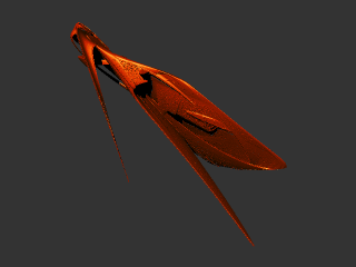 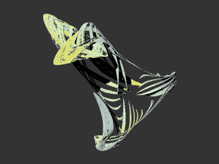 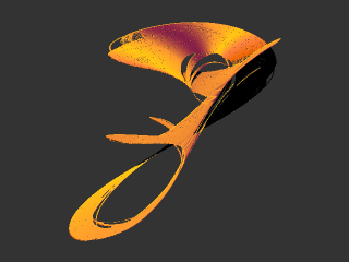 |
| Pickover |
|---|
|
The algorithm used to calculate the new x, y and z points is xnew=sin(a3da[0]*y)-z*cos(a3da[1]*x) ynew=z*sin(a3da[2]*x)-cos(a3da[3]*y) znew=a3da[4]*sin(x) Here are some sample images created using this attractor type 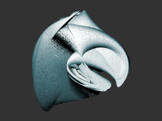 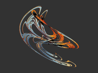 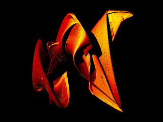 |
| Polynomial A |
|---|
|
The algorithm used to calculate the new x, y and z points is xnew=a3da[0]+y-z*y ynew=a3da[1]+z-x*z znew=a3da[2]+x-y*x Here are some sample images created using this attractor type 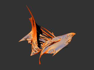 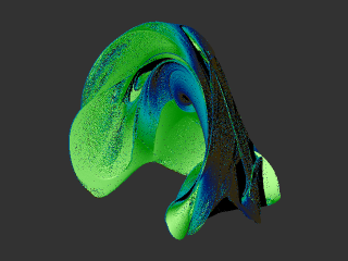 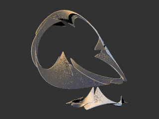 |
| Polynomial B |
|---|
|
The algorithm used to calculate the new x, y and z points is xnew=a3da[0]+y-z*(a3da[1]+y) ynew=a3da[2]+z-x*(a3da[3]+z) znew=a3da[4]+x-y*(a3da[5]+x) Here are some sample images created using this attractor type 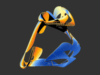 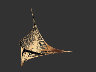 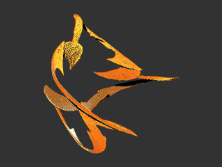 |
| Polynomial C |
|---|
|
The algorithm used to calculate the new x, y and z points is xnew=a3da[0]+x*(a3da[1]+a3da[2]*x+a3da[3]*y)+y*(a3da[4]+a3da[5]*y) ynew=a3da[6]+y*(a3da[7]+a3da[8]*y+a3da[9]*z)+z*(a3da[10]+a3da[11]*z) znew=a3da[12]+z*(a3da[13]+a3da[14]*z+a3da[15]*x)+x*(a3da[16]+a3da[17]*x) Here are some sample images created using this attractor type 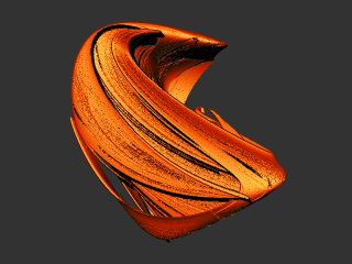 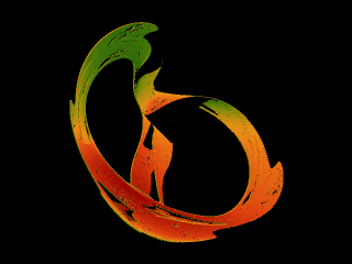 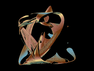 |
| Polynomial ABS |
|---|
|
The algorithm used to calculate the new x, y and z points is xnew=a3da[0] + a3da[1]*x + a3da[2]*y + a3da[3]*z + a3da[4]*abs(x) + a3da[5]*abs(y) +a3da[6]*abs(z) ynew=a3da[7] + a3da[8]*x + a3da[9]*y + a3da[10]*z + a3da[11]*abs(x) + a3da[12]*abs(y) +a3da[13]*abs(z) znew=a3da[14] + a3da[15]*x + a3da[16]*y + a3da[17]*z + a3da[18]*abs(x) + a3da[19]*abs(y) +a3da[20]*abs(z) Here are some sample images created using this attractor type 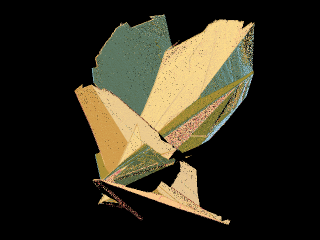 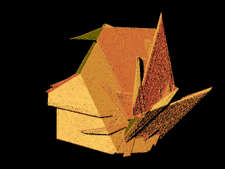 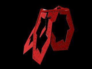 |
| Polynomial Power |
|---|
|
The algorithm used to calculate the new x, y and z points is xnew=a3da[0] + a3da[1]*x + a3da[2]*y + a3da[3]*z + a3da[4]*abs(x) + a3da[5]*abs(y) +a3da[6]*power(abs(z),a3da[7]) ynew=a3da[8] + a3da[9]*x + a3da[10]*y + a3da[11]*z + a3da[12]*abs(x) + a3da[13]*abs(y) +a3da[14]*power(abs(z),a3da[15]) znew=a3da[16] + a3da[17]*x + a3da[18]*y + a3da[19]*z + a3da[20]*abs(x) + a3da[21]*abs(y) +a3da[22]*power(abs(z),a3da[23]) Here are some sample images created using this attractor type 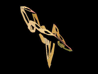 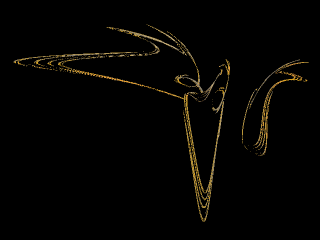 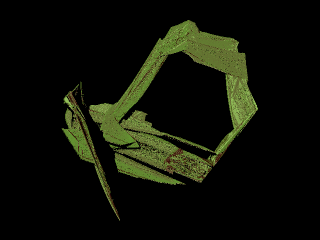 |
| Polynomial Sin |
|---|
|
The algorithm used to calculate the new x, y and z points is xnew=a3da[0] + a3da[1]*x + a3da[2]*y + a3da[3]*z + a3da[4]*sin(a3da[5]*a3da[6]*x) + a3da[7]*sin(a3da[8]*a3da[9]*y) +a3da[10]*sin(a3da[11]*a3da[12]*z) ynew=a3da[13] + a3da[14]*x + a3da[15]*y + a3da[16]*z + a3da[17]*sin(a3da[18]*a3da[19]*x) + a3da[20]*sin(a3da[21]*a3da[22]*y) +a3da[23]*sin(a3da[24]*a3da[25]*z) znew=a3da[26] + a3da[27]*x + a3da[28]*y + a3da[29]*z + a3da[30]*sin(a3da[31]*a3da[32]*x) + a3da[33]*sin(a3da[34]*a3da[35]*y) +a3da[36]*sin(a3da[37]*a3da[38]*z) Here are some sample images created using this attractor type 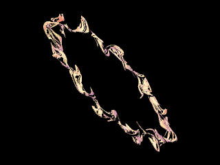 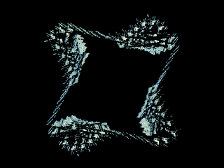 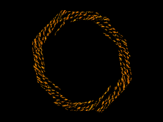 |
| Rampe 1 |
|---|
|
The algorithm used to calculate the new x, y and z points is xnew=z*sin(a3da[0]*x)+cos(a3da[1]*y) ynew=x*sin(a3da[2]*y)+cos(a3da[3]*z) znew=y*sin(a3da[4]*z)+cos(a3da[5]*x) Here are some sample images created using this attractor type 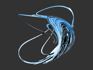 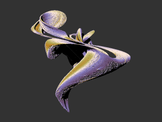 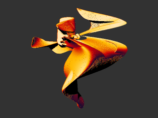 |
| Rampe 2 |
|---|
|
The algorithm used to calculate the new x, y and z points is xnew=z*sin(a3da[0]*x)+arccos(a3da[1]*y) ynew=x*sin(a3da[2]*y)+arccos(a3da[3]*z) znew=y*sin(a3da[4]*z)+arccos(a3da[5]*x) Here are some sample images created using this attractor type  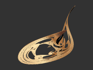 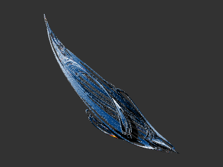 |
| Rampe 3 |
|---|
|
The algorithm used to calculate the new x, y and z points is xnew=x*z*sin(a3da[0]*x)-cos(a3da[1]*y) ynew=y*x*sin(a3da[2]*y)-cos(a3da[3]*z) znew=z*y*sin(a3da[4]*z)-cos(a3da[5]*x) Here are some sample images created using this attractor type 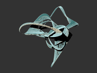 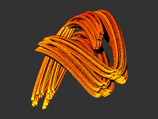 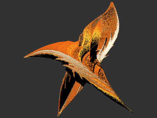 |
| Rampe 4 |
|---|
|
The algorithm used to calculate the new x, y and z points is xnew=x*sin(a3da[0]*x)+cos(a3da[0]*y) ynew=y*sin(a3da[1]*y)+cos(a3da[1]*z) znew=z*sin(a3da[2]*z)+cos(a3da[2]*x) Here are some sample images created using this attractor type 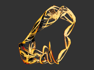 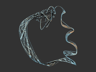 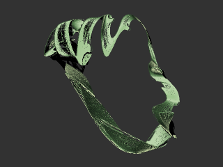 |
| Rampe 5 |
|---|
|
The algorithm used to calculate the new x, y and z points is xnew=y*sin(a3da[0]*x)+cos(a3da[1]*y)+sin(a3da[2]*z) ynew=z*sin(a3da[3]*x)+cos(a3da[4]*y)+sin(a3da[5]*z) znew=x*sin(a3da[6]*x)+cos(a3da[7]*y)+sin(a3da[8]*z) Here are some sample images created using this attractor type 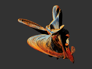 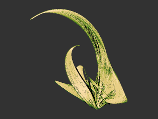 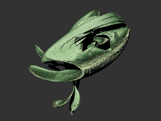 |
| Rampe 6 |
|---|
|
The algorithm used to calculate the new x, y and z points is xnew=z*sin(a3da[0]*x)-cos(a3da[1]*y) ynew=x*sin(a3da[2]*y)+cos(a3da[3]*z) znew=y*sin(a3da[4]*z)-cos(a3da[5]*x) Here are some sample images created using this attractor type 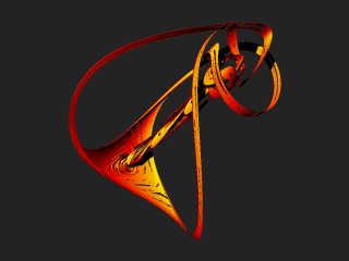  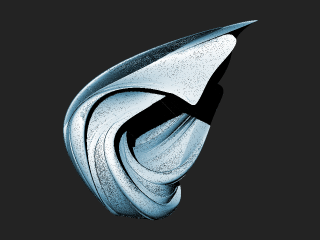 |
| Rampe 7 |
|---|
|
The algorithm used to calculate the new x, y and z points is xnew=z*sin(a3da[0]*x)-cos(a3da[1]*y) ynew=x*cos(a3da[2]*y)+sin(a3da[3]*z) znew=y*sin(a3da[4]*z)-cos(a3da[5]*x) Here are some sample images created using this attractor type 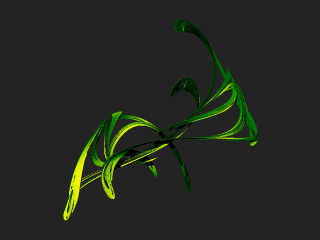 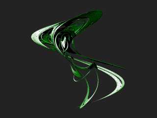 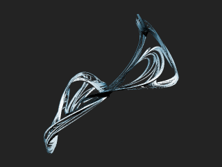 |
| Rampe 8 |
|---|
|
The algorithm used to calculate the new x, y and z points is xnew=z*sin(a3da[0]*x)-cos(y) ynew=x*cos(a3da[1]*y)+sin(z) znew=y*sin(a3da[2]*z)-cos(x) Here are some sample images created using this attractor type 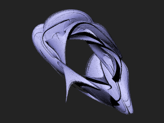 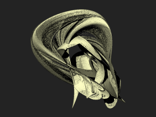 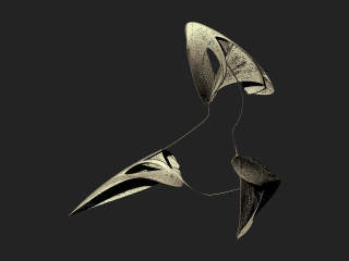 |
| Rampe 9 |
|---|
|
The algorithm used to calculate the new x, y and z points is xnew=y*sin(a3da[0]*x)-arccos(a3da[1]*y)+sin(a3da[2]*z) ynew=z*sin(a3da[3]*x)-arccos(a3da[4]*y)+sin(a3da[5]*z) znew=x*sin(a3da[6]*x)-arccos(a3da[7]*y)+sin(a3da[8]*z) Here are some sample images created using this attractor type 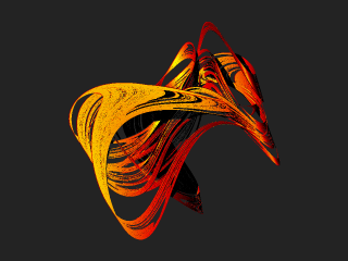 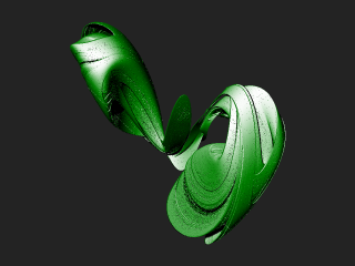 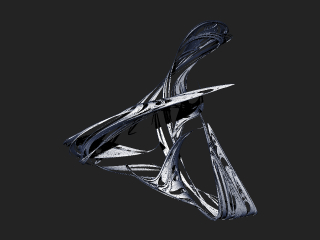 |
| Rampe 10 |
|---|
|
The algorithm used to calculate the new x, y and z points is xnew=y*sin(a3da[0]*x)-cos(a3da[1]*y)+arcsin(a3da[2]*z) ynew=z*sin(a3da[3]*x)-cos(a3da[4]*y)+sin(a3da[5]*z) znew=x*sin(a3da[6]*x)-cos(a3da[7]*y)+sin(a3da[8]*z) Here are some sample images created using this attractor type 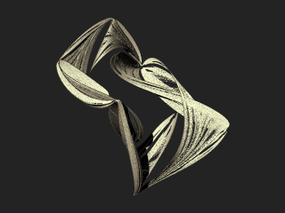 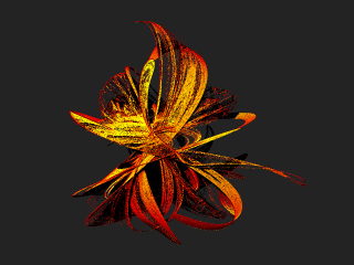 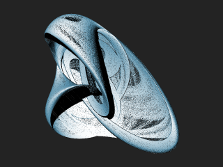 |
| Other Settings |
|---|
Display Style - Hit Count - Colors the attractor by the number of times each pixel is hit as the formula iterates. This gives more of a 2D attractor style render.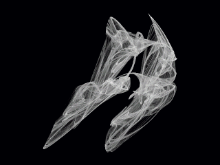 Display Style - Depth - Colors each pixel depending on its depth in 3D space. 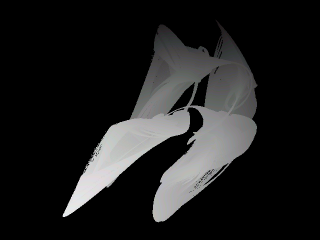 Display Style - Solid - Shades and shadows the attractor to give a more 3D appearance. 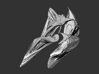 Background color - Allows any color to be used as the background around the attractor. Shadows - Enables or disables shadows on the attractor surface. Shadows help to bring out the 3D details. Rotation - Degrees between 0 and 360 that the attractor is rotated. Attractors usually have a completely different look from other angles. Tip: To create an AVI movie of a 3D strange attractor rotating, select Frames->Create Frames and then change the Frame Generation Style to 360 Degree 3D Rotation.Supersample - Increases the detail of the resulting image and smooths out the pixelated appearance. Render to BMP - Creates a bitmap image of the current attractor. This can be set to an image size larger than the current screen resolution. Save button - Allows the current settings to be saved for future use. Load button - Loads a previous settings file. Visions Of Chaos includes a series of sample 3D Attractor files. Mutate button - Opens a dialog that creates a new set of images based on the current settings. This can help tweak an attractor by changing the parameters slightly and finding a more pleasing result. Background Image - If an image is selected then the image will replace the background color and appear behind the rendered attractor. |